TP3 : B-splines, De Boor's algorithm
Code
Update your local repo
git pull
or clone everything if needed
git clone https://github.com/bbrrck/geo-num-2016.git
As usual,
cd TP3/
mkdir build
cd build
cmake ..
make
./geonum_TP3 simple
We’re still using Eigen so keep the quick reference open and ready.
Python script for rendering is included in the plots/ folder.
You can now pass the data name as an argument
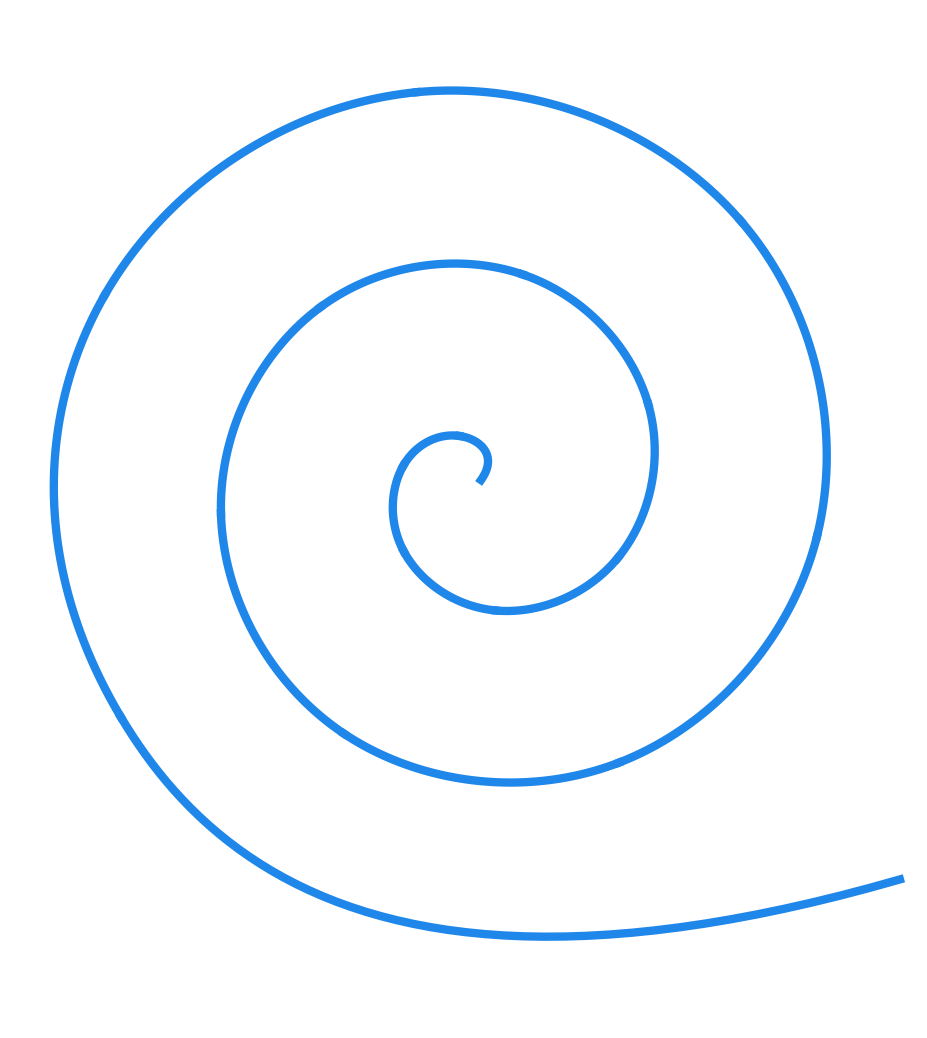
python ../plots/plot.py spiral
If you want to use gnuplot, you will need to modify the script from TP1 yourself.
B-splines
Given the degree $k$, $n+1$ control points $\mathbf d_0,\dots,\mathbf d_n$, and the knot vector $t_0 \leq t_1 \leq \dots \leq t_m$ with $m = n+k+1$, the B-spline curve $S(t)$ is defined as
\[S(t) = \sum_{j=0}^n \mathbf d_j N_j^k(t), \quad t\in[t_k, t_{n+1}).\]The $N_j^k$ are the recursively-defined basis functions (hence the name B-spline)
\[\begin{array}{ll} N_j^{0}(t) =& \begin{cases} 1 \quad t\in[t_j, t_{j+1}) \\ \\ 0 \quad \text{ otherwise } \end{cases} \\ \\ N_j^k(t) =& \underbrace{ \frac{ t - t_j }{ t_{j+k} - t_j } }_{ w_{j,k}(t)} N_j^{k-1}(t) + \underbrace{ \frac{ t_{j+k+1} - t}{ t_{j+k+1} - t_{j+1} } }_{1 - w_{j+1,k}(t)} N_{j+1}^{k-1}(t) \end{array}\]Looks complicated? Don’t worry if you cannot get your head around all the indices and whatnot; De Boor is here to help you!
B-spline basis functions $N^k_j$ up to degree 5 for the knot sequence $(0,1,2,3,4,5,6,7)$.
De Boor’s algorithm
… also called the De Boor-Cox algorithm. It can be seen as the generalization of the de Casteljau. (A Bézier curve is in fact a special case of B-spline.)
- input :
degree $k$
$n+1$ control points $\mathbf{d_{0}},\dots,\mathbf{d_{n}}$
knot vector $t_0 \leq t_1 \leq \dots \leq t_m$ with $m = n+k+1$
parameter $t \in [t_i, t_{i+1}) \quad k \leq i \leq n$ - output : The point $\mathbf S(t) = \mathbf d_j^k$ on the curve.
- compute : For $j=i-k, \dots, i,$ set $\mathbf d_j^0 = \mathbf d_j$. Then compute the points \begin{align} \mathbf d_{j}^{r} &= (1-w_{j,k-(r-1)}) \mathbf d_{j-1}^{r-1} + w_{j,k-(r-1)} \mathbf d_{j }^{r-1} \end{align} for \begin{align} \quad r = 1,\dots,k, \quad \quad j = i-k+r,\dots,i \end{align} with \begin{align} w_{j,k-(r-1)} &= \frac{ t - t_j }{ t_{j+k-(r-1)} - t_j }. \end{align}
Be careful with the indices! Here I’ve expressed the point at depth $r$ in terms of the points at depth $r-1$; that is why there is the $r-1$ everywhere in the formula. (It becomes much more elegant if we express $r+1$ in terms of $r$.) This might be a bit annoying, but I think it’s also more practical for the implementation.
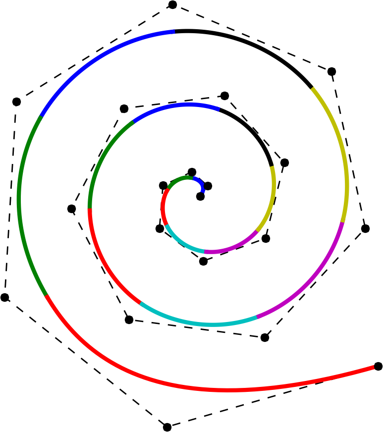
A cubic B-spline with 16 segments and endpoint interpolation.
ToDo
- Implement the De Boor’s algorithm. (
Vec2 DeBoor) - Implement the evaluation of a B-spline curve. (
evaluateBSpline) - Compute the B-spline curve for the
simpledataset. Then, modify the knot vector and recompute. What happened? - Compute the B-spline curve for the
spiraldataset. Try using the knot vector0 0 0 0 1 1 1 1 2 2 2 2 3 3 3 3 4 4 4 4 5 5 5 5. What changed? - Compute the B-spline curve for the
cameldataset. Move the front leg by changing the x-coordinate of the very last control point to-1.5. Which segments of the curve have changed? Why?
NURBS
If you’ve done the tests with the circle.bspline dataset, you might have been disappointed,
as the resulting curve is far from being a nice circle.
The truth is, it’s mathematically impossible to represent the unit circle as a B-spline.
However, it is possible (and not so hard) using a further generalization of the B-spline curves: the non-uniform rational B-splines or NURBS.
If you examine the circle.nurbs file, you’ll find it’s not so different from the circle.bspline.
The only thing that’s changed is the additional number after each control point.
It almost looks like the control points don’t live in 2D, but in 3D.
If that thought occured to you, you’re not far from the truth:
together, those three numbers define the homogeneous (or projective) coordinates of a control point.
The third number is often called a weight of the control point.
Here’s the good news: even with the homogeneous coordinates, we can apply exactly the same De Boor’s algorithm without any modifications. So, if you’re up for it, here’s a secret recipe for transforming your 2D B-splines into 2D NURBS:
-
Use a matrix of type
MatX3to store the control points (the first and second column are the x and y coordinates, respectively; the third column hold the weights). For reading thecircle.nurbsfile, you can still use the methodreadBSpline, no change here; just make sure the second argument you pass is a three-column matrix. Let’s call this matrixControlPoints3. -
DeBoor3:you can copy-paste everything from the 2D version, just be sure to change the types toVec3andMatX3. -
Before you begin the evaluation, you need to multiply the x and y coordinates (first two columns of the
ControlPoints3matrix) by the weights (third column). You can do this withControlPoints3.col(i) = ControlPoints3.col(i).array() * ControlPoints3.col(2).array();fori=0,1.The.array()tells the Eigen to perform the operation element-wise. -
Proceed by evaluating the
SplinePoints3with three coordinates. -
The last step is to return to the plane coordinates. To do that, you need to divide by the weights. Much like before, this is done with
SplinePoints2.col(i) = SplinePoints3.col(i).array() / SplinePoints3.col(2).array();
Bonus ToDo
- Implement the NURBS curve by extending your B-spline methods.
- Compute and visualise the circle as a NURBS curve.
Resources
- B-spline and De Boor’s algorithm
- 1.4.2 B-spline curve and 1.4.3 Algorithms for B-spline curves, online chapters from the book Shape Interrogation for Computer Aided Design and Manufacturing by N. Patrikalakis, T. Maekawa & W. Cho
- NURBS on wikipedia (includes the circle example)
- homepage of Prof. de Boor