TP7 : B-spline Surfaces

25 March 2016 in

Code

git pull

or, if you don’t have the local repo,

git clone https://github.com/bbrrck/geo-num-2016.git

As usual, test by

cd TP7/
mkdir build
cd build
cmake ..
make

To test the viewer, try running

./geonum_TP7 simple

If everything goes well, you should see a cube. The viewer can be controlled with the mouse: click and drag to rotate, scroll to zoom (also works with pageup/pagedown keys).

In case the SimpleViewer does not work, you can still export and visualise the surfaces via the python script, included in plots/.

B-spline curves revisited

Back in TP3, we were working with B-spline curves. A B-spline curved is defined by the following:

$k : \text{ degree } \\ \mathbf d_{0},\dots, \mathbf d_{n} : \text{ control polygon } \\ t_{0},\dots,t_{m+k+1} : \text{ knot vector }$

Tensor product B-spline surfaces

A B-spline surface is defined via

$k, l : \text{ degrees in } u, v \\ \text{ } \\ \left( \begin{array}{ccc} \mathbf d_0^0 & \dots & \mathbf d_m^0 \\ \vdots & \ddots & \vdots \\ \mathbf d_0^n & \dots & \mathbf d_m^n \end{array} \right) : \text{ control net } \\ \text{ } \\ u_0,\dots,u_{m+k+1} : \text{ knot vector in } u \\ v_0,\dots,v_{n+l+1} : \text{ knot vector in } v$

The B-spline surface is defined for $(u,v) \in [u_k,u_{m+1}] \times [v_l,v_{n+1}]$ as

$S(u,v) = \sum_{i=0}^m \sum_{j=0}^n \mathbf d_i^j N_{i}^{k}(u) N_{j}^{l}(v).$

Surface Patches

Recall that a B-spline curve is made from many smaller pieces, defined over parameter intervals $[t_i,t_{i+1}]$. Analogically, a B-spline surface consists of $(m-k+1) \times (n-l+1)$ patches, each defined over a parameter rectangle $[u_i,u_{i+1}] \times [v_j,v_j+1]$ :

$\begin{array}{llll} [u_{k},u_{k+1}] \times [v_{l },v_{l+1}] & [u_{k+1},u_{k+1}] \times [v_{l },v_{l+1}] & \dots & [u_{m},u_{m+1}] \times [v_{l },v_{l+1}] \\ [u_{k},u_{k+1}] \times [v_{l+1},v_{l+2}] & [u_{k+1},u_{k+1}] \times [v_{l+1},v_{l+2}] & \dots & [u_{m},u_{m+1}] \times [v_{l+1},v_{l+2}] \\ \vdots & \vdots & \ddots & \vdots \\ [u_{k},u_{k+1}] \times [v_{n-1},v_{n }] & [u_{k+1},u_{k+1}] \times [v_{n-1},v_{n }] & \dots & [u_{m},u_{m+1}] \times [v_{n-1},v_{n }] \\ [u_{k},u_{k+1}] \times [v_{n },v_{n+1}] & [u_{k+1},u_{k+1}] \times [v_{n },v_{n+1}] & \dots & [u_{m},u_{m+1}] \times [v_{n },v_{n+1}] \\ \end{array}$

Each patch needs to be evaluated individually, then stored in one big matrix (per coordinate).

Evaluation

To evaluate a point on a B-spline surface, use the same principle as in the last TP: first, evaluate in the $u$ direction $n+1$ times; then use the computed points as the control polygon for a curve in the $v$ direction. As always, this can be done iteratively or recursively. A recursive implementation of the DeBoor’s algorithm is included in todo.h; however, it is strongly advised to use you own (from TP3).

We will use the same paradigm as in the previous TP, i.e. the points will be stored coordinate-wise; in matrices X, Y, Z (or netX, netY, netZ for the control net).

Algorithm

The implementation of a B-spline surface can be summarized in the following pseudocode.

# loop over all patches
for i in (k,k+1,...,m) :
    for j in (l,l+1,...,n) :
        # loop over the samples of the current patch
        # defined over [u_i,u_{i+1}] x [v_j,v_{j+1}]
        for u in uniform_sampling( u_{i}, u_{i+1}, number_of_samples ) :
            for v in uniform_sampling( v_{j}, v_{j+1}, number_of_samples ) :
                compute_S(u,v) # a surface point on the current patch

ToDo

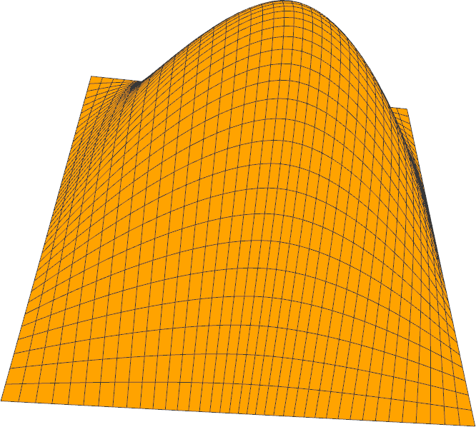
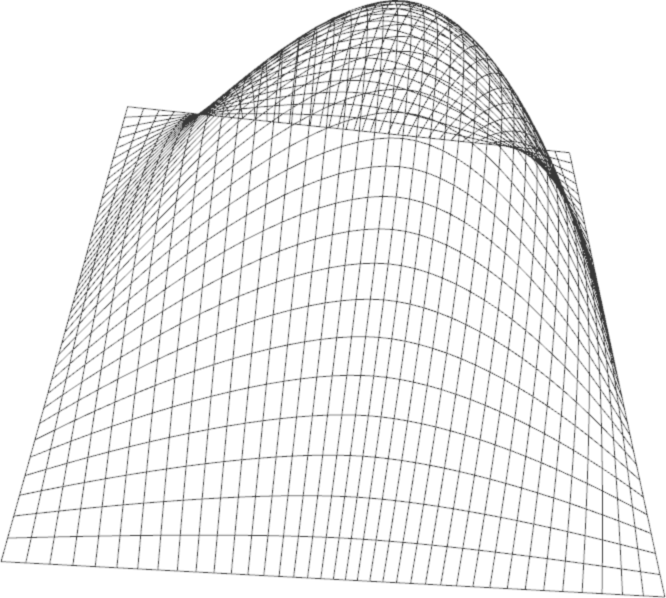
Implement the evaluation of B-spline surfaces.
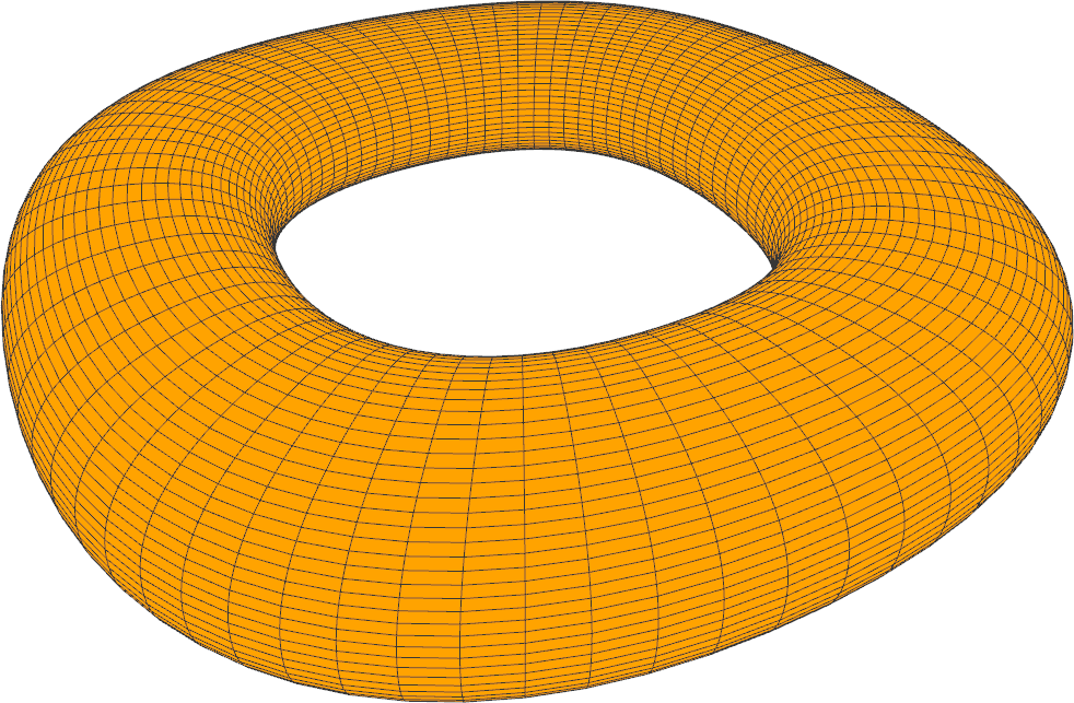
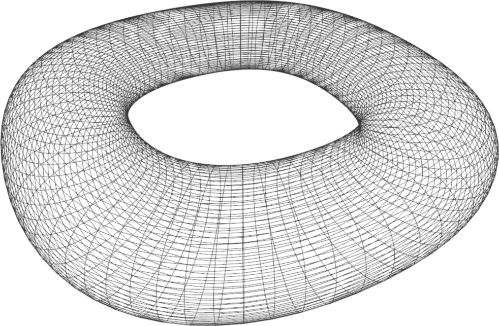
Modify the knot vectors for the simple dataset. Experiment with various configurations. How does the surface change?
[Bonus] A NURBS surface (Non-Uniform Rational B-Spline) can be used to represent a sphere, the same way we used a NURBS curve to represent the unit circle in TP3. Modify your implementation of B-spline surfaces in order to compute a NURBS surface. The control points and weights for representing a sphere can be found in Representing a Circle or a Sphere with NURBS by David Eberly.

simple full simple wire

torus full torus wire

Resources

B-spline surfaces : Construction
1.4.4 B-spline surface, online chapters from the book Shape Interrogation for Computer Aided Design and Manufacturing by N. Patrikalakis, T. Maekawa & W. Cho
NURBS on wikipedia