TP1 : Bézier curves, De Casteljau’s algorithm
Bézier curves
A degree $n$ Bézier curve takes the form
\[\mathbf x(t) = \sum_{i=0}^{n} \mathbf b_i B_i^n(t) \qquad t \in [0,1]\]where
\[B_{i}^{n}(t) = \begin{pmatrix}n \\ i\end{pmatrix} (1-t)^{n-i} t^i\]are the degree $n$ Bernstein polynomials, and the binomial coefficients are defined as
\[\begin{pmatrix}n \\ i\end{pmatrix} = \frac{n!}{(n-i)! i!}.\]The Bézier points $\mathbf b_i \in \mathbb R^d$ form the control polygon.
De Casteljau’s algorithm
- input Bézier points $\mathbf b_i$ for $i = 0, \dots, n$, and parameter $t \in [0,1]$.
- output The point $\mathbf b_0^n$ on the curve.
-
compute Set $\mathbf b_i^0 = \mathbf b_i$ and compute the points
\[\mathbf b_i^k (t) = (1-t) \mathbf b_i^{k-1} + t \mathbf b_{i+1}^{k-1} \qquad \text{for} \qquad k=1,\dots,n, \quad i=0,\dots,n-k.\]
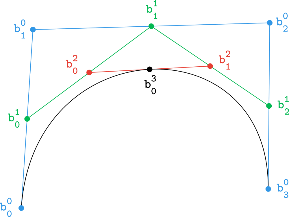
Visualisation of the steps of the De Casteljau’s algorithm, $t=0.5$.
The De Casteljau’s algorithm provides an efficient means for evaluating a Bézier curve $\mathbf{x}(t)$. It is useful to look at this algorithm in its schematic form. For a cubic curve ($n=3$):
\[\begin{array}{ccccccc} \mathbf b_0 = \mathbf b_0^0 & & & & & & \\ & \ddots & & & & & \\ \mathbf b_1 = \mathbf b_1^0 & \dots & \mathbf b_0^1 & & & & \\ & \ddots & & \ddots & & & \\ \mathbf b_2 = \mathbf b_2^0 & \dots & \mathbf b_1^1 & \dots & \mathbf b_0^2 & & \\ & \ddots & & \ddots & & \ddots & \\ \mathbf b_3 = \mathbf b_3^0 & \dots & \mathbf b_2^1 & \dots & \mathbf b_1^2 & \dots & \mathbf b_0^3 = \mathbf x(t) \end{array}\]
Animation of the De Casteljau’s algorithm for a quintic curve ($n=5$).
Code
ToDo
- Implement the De Casteljau algorithm and use it to evaluate the Bézier curves in the
datafolder. Visualise the curves together with their control polygons. - Try varying the sampling density. How many samples are needed to give the impression of a smooth curve?
- Pick one dataset and visualise all intermediate polygons $\mathbf b_i^k$ from the De Casteljau algorithm for a fixed parameter, for instance $t=0.5$.
Hint: each column in the above schema represents one such polygon.
Resources
- Handbook of CAGD, edited by Gerald Farin, Josef Hoschek, Myung-Soo Kim
- A Primer on Bézier Curves by Pomax
- Bézier Curves and Picasso by Jeremy Kun
- Bézier Curves and Type Design: A Tutorial by Fábio Duarte Martins
- The Bézier Game
- Bézier Curve Simulation