TP2 : Bézier splines, $C^k$ smoothness
Code
Bézier splines
Bézier curves become harder to work with as the number of control points gets bigger. The main reason is their global nature – moving a single control point influences the whole curve. Do you know why? (Hint: take a look at the De Casteljau schema in the previous TP.)
Also, more control points means higher-degree polynomial, which quickly becomes impractical. Today, we’ll be dealing with one possiblity on how to overcome this problem: the Bézier splines.
Informally, spline is a collection of curves connected with some degree of smoothness. There is more than one way to define what does it mean for two curves to be smoothly connected. The most commonly used is the $\mathcal C^k$ smoothness.
$\mathcal C^k$ smoothness
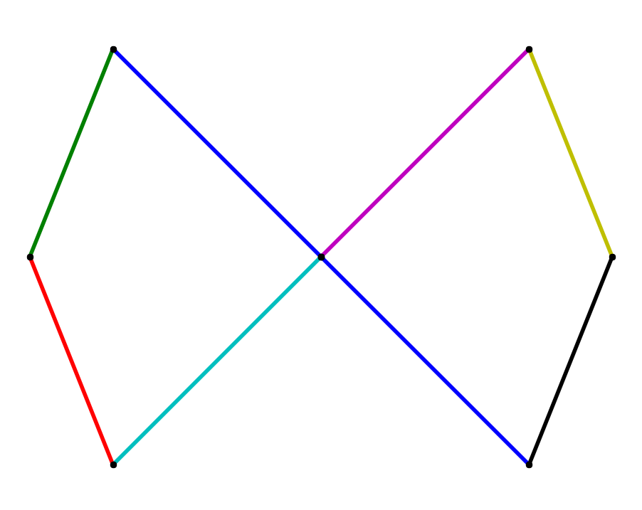
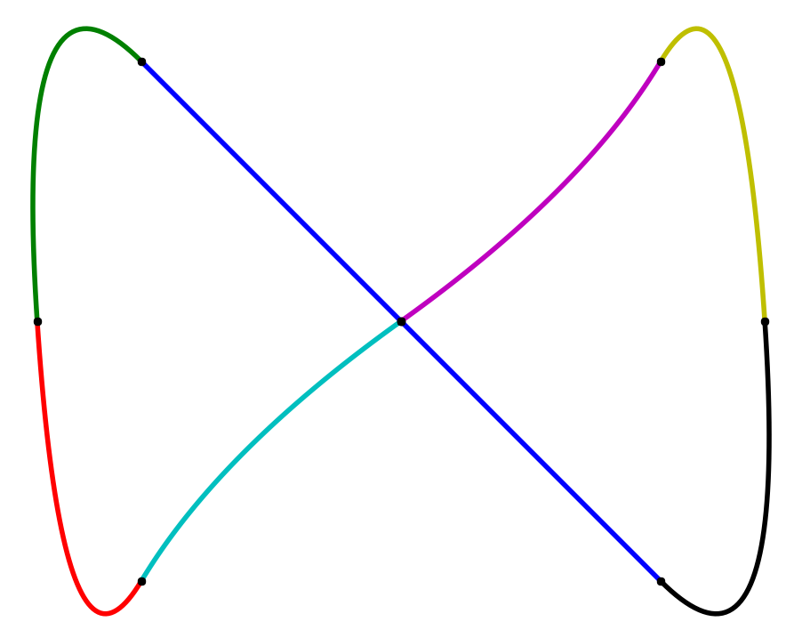
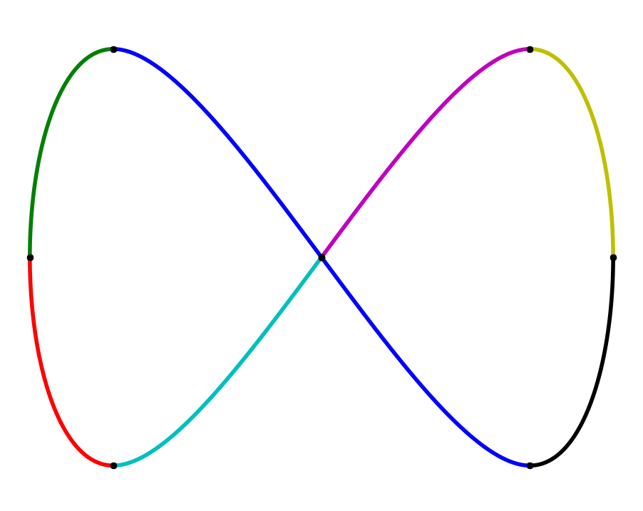
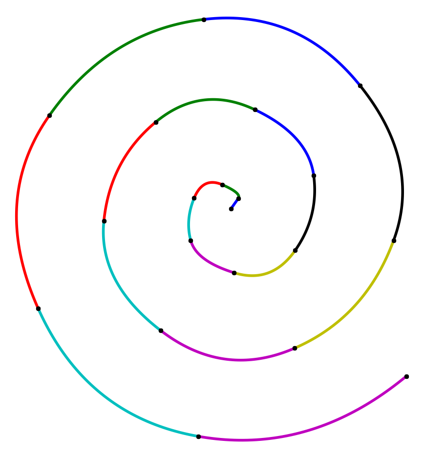
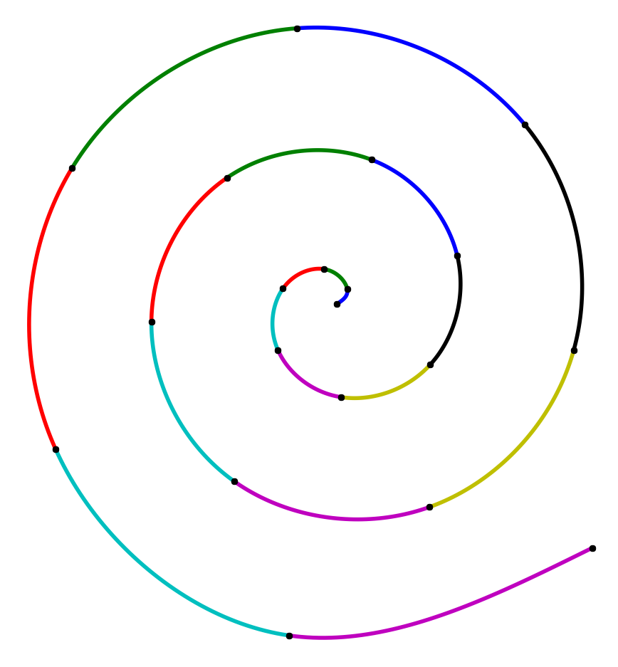
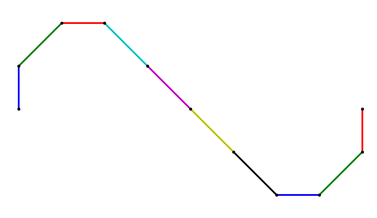
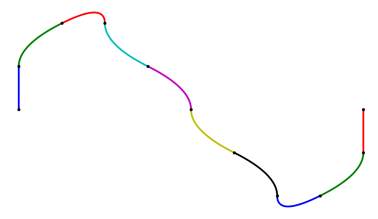
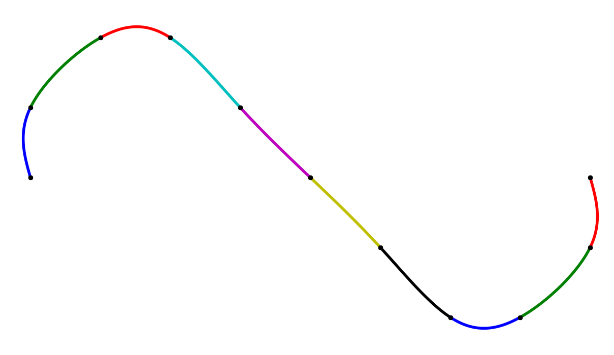
A collection of $ \mathcal C^k$-smooth splines, row-wise interpolating the same data, left to right $k=0,1,2$.
Mathematically speaking, two parametric curves $\mathbf x_0(t), \mathbf x_1(t), t \in [0,1]$ are $\mathcal C^k$ smooth if they are also $\mathcal C^{k-1}$, and the following condition holds:
\[\frac{d^k}{dt^k} \mathbf x_0\left(1\right) = \frac{d^k}{dt^k} \mathbf x_1\left(0\right),\]meaning the two curves agree up to their $k$-th derivatives. Let’s look at a particular case when $\mathbf x_0$ and $\mathbf x_1$ are Bézier curves.
$\mathcal C^1$ quadratic spline
Recall that a quadratic Bézier curve has the form
\[\mathbf x(t) = \sum_{i=0}^{2} \mathbf b_i B_i^2(t) \qquad t \in [0,1]\]where $\mathbf b_i$ are the control points and $B_i^2(t)$ are the quadratic Bernstein polynomials. Its first derivative $\dot{\mathbf x} = \frac{d^2}{dt^2} \mathbf x$ can be nicely written as
\[\dot{\mathbf x}(t) = n \sum_{i=0}^{1} (\mathbf b_{i+1} - \mathbf b_i) B_i^{1}(t) = (1-t)(\mathbf b_2 - \mathbf b_1) + t(\mathbf b_1 - \mathbf b_0).\]In fact, the derivative is also a Bézier curve, of degree $n-1$.
Now, imagine the two Bézier curves $\mathbf x_0, \mathbf x_1$ are to be joined $\mathcal C^1$-smoothly. As $\mathcal C^1$ also includes $\mathcal C^0$, we have two conditions:
\[\begin{align} \mathbf x_0(1) &= \mathbf x_1(0), \\ \dot{\mathbf x}_0(1) &= \dot{\mathbf x}_1(0). \end{align}\]If $\mathbf b_i^0$ are the control points of $\mathbf x_0$, and $\mathbf b_i^1$ are the control points of $\mathbf x_1$, this comes down to
\[\begin{align} \mathbf b_2^0 &= \mathbf b_0^1, \\ \mathbf b_2^0 - \mathbf b_1^0 &= \mathbf b_1^1 - \mathbf b_0^1. \end{align}\]ToDo$^1$
Your first task today will be to implement $\mathcal C^1$ quadratic Bézier spline, interpolating a given sequence of points $\mathbf p_i, i=0,\dots,n$. To construct the spline, you’ll need $n$ quadratic Bézier curves $\mathbf x_i, i=0,\dots,n-1$, each with three control points: $\mathbf p_{i} = \mathbf b_0^i, \mathbf b_1^i, \mathbf b_2^i = \mathbf p_{i+1}$. (Don’t get confused: here, the upper indices have nothing to do with de Casteljau!) This means that for each curve, you only need to compute a single control point $\mathbf b_1^i$. Applying the formula from above for the joint between $\mathbf x_i$ and $\mathbf x_{i+1}$ we get
\[\mathbf b_2^{i} - \mathbf b_1^{i} = \mathbf b_1^{i+1} - \mathbf b_0^{i+1}\]and from there, directly
\[\begin{align} \mathbf b_1^{i+1} &= \mathbf b_2^{i} - \mathbf b_1^{i} + \mathbf b_0^{i+1} \\ &= 2 \mathbf p_{i+1} - \mathbf b_1^{i} . \end{align}\]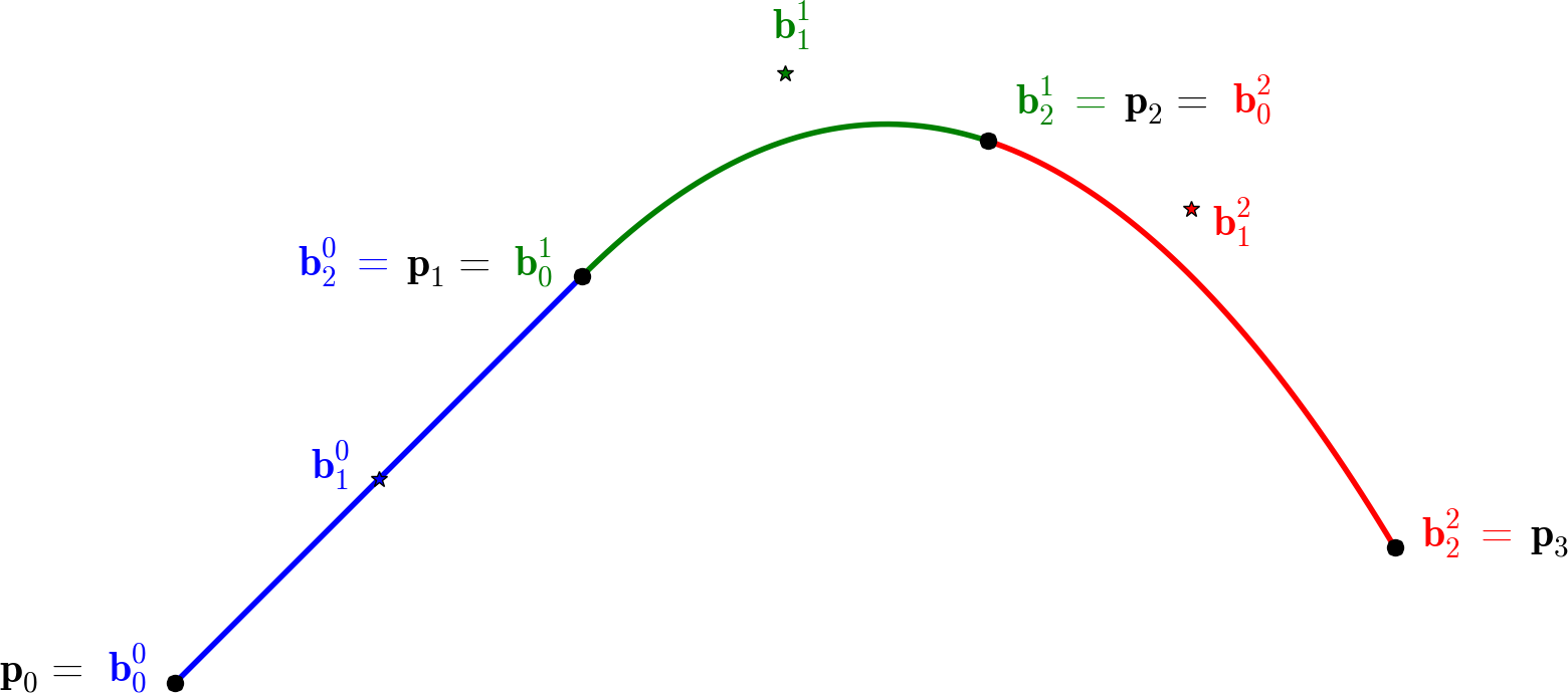
This gives us an iterative way to compute all of $\mathbf b_1^i$.
You will need to manually fix $\mathbf b_1^0$. Try the midpoint $0.5(\mathbf p_0 + \mathbf p_1)$; later, you can change its position to see how it affects the computed spline.
- Implement the computation of control points of a quadratic interpolating Bézier spline for a given sequence of points $\mathbf p_i$ (function
ComputeSplineC1). Evaluate and visualise for the available datasets. - Try changing the position of $\mathbf b_1^0$. What happens?
$\mathcal C^2$ cubic spline
Splines, especially the cubic splines, are very common in the world of digital geometry. The algorithm you just implemented (hopefully) works well, but it has one major drawback: it requires setting the first $\mathbf b_1^0$ by hand. That’s no fun!
That is why, to compute an interpolating cubic spline in this part, we will adopt a slightly different approach – by solving a linear system. We’ll do the math, crunch in the data, and let the solver do the work.
To do that, take a situation much like the one before: given a sequence of points $\mathbf p_i, i=0,\dots,n$, find a $\mathcal C^2$ cubic spline (i.e. $n$ cubic curves) which interpolates these datapoints. This time, there will be two unknown interior control points for each curve, not one as in the quadratic case.
Again, let’s take only two cubic curves to understand what’s going on; $\mathbf x_0$ with control points $\mathbf b_i^0$ and $\mathbf x_1$ with control points $\mathbf b_i^1$. $\mathcal C^2$ means also $\mathcal C^1$: but we already know how to write $\mathcal C^1$ in terms of control points! Let’s add the $\mathcal C^2$:
\[\begin{align} \mathbf b_3^0 &= \mathbf b_0^1 \\ \mathbf b_3^0 - \mathbf b_2^0 &= \mathbf b_1^1 - \mathbf b_0^1 \\ \mathbf b_3^0 - 2\mathbf b_2^0 + \mathbf b_1^0 &= \mathbf b_2^1 - 2\mathbf b_1^1 + \mathbf b_0^1 \\ \end{align}\]Well, it’s starting to look like a system, but all this indexing is confusing. So let’s take a step back.
Imagine we want to interpolate four points, i.e. we have three curves to compute. That’s 10 unique control points in total. We’ll denote those as $A,B,C,D,E,F,G,H,I,J$. (Phew.) The points to interpolate are $A,D,G,J$.
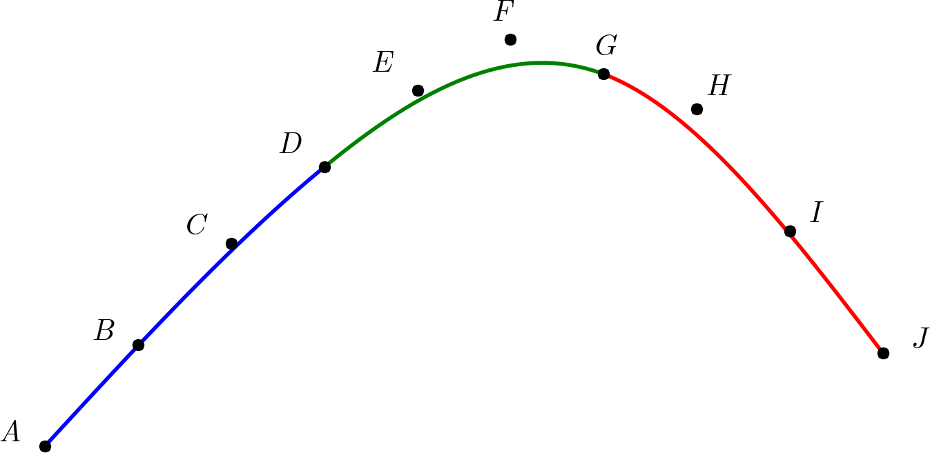
Let’s rewrite our conditions in terms of this notation.
$\mathcal C^0$:
\[\begin{align} A = & A \\ D = & D \\ G = & G \\ J = & J \end{align}\]Seems pretty obvious, right? We have two joints, that means two equations for $\mathcal C^1$:
\[\begin{align} D - C =& E - D \\ G - F =& H - G \end{align}\]And two equations for $\mathcal C^2$:
\[\begin{align} D - 2C + B =& F - 2E + D \\ G - 2F + E =& I - 2H + G \end{align}\]If you’ve counted well, this makes 8 equations for 10 points; we need two more equations to be able to solve the system. (In general, this is $(n+1)+(n-1)+(n-1)=3n-1$ equations for $3n+1$ points and we still need two more equations.) One example is the so-called natural spline with vanishing second derivatives at the endpoints, i.e. \(\ddot{\mathbf x}_0(0) = \mathbf 0 = \ddot{\mathbf x}_{n-1}(1)\):
\[\begin{align} A - 2B + C =& \mathbf 0 \\ H - 2I + J =& \mathbf 0 \end{align}\]where $\mathbf 0 = (0,0)$ is the zero vector. And that’s it! Everything’s much clearer using the matrix notation (blank spaces indicate zeros):
\[\left[ \begin{array}{rr|rr|rr|rr|rr} 1 & & & & & & & & & \\ & & & 1 & & & & & & \\ & & & & & & 1 & & & \\ & & & & & & & & & 1 \\ \hline & & 1 & -2& 1 & & & & & \\ & & & & & 1 & -2& 1 & & \\ \hline & 1 &-2 & & 2 & -1& & & & \\ & & & & 1& -2& & 2 &-1 & \\ \hline 1 & -2& 1 & & & & & & & \\ & & & & & & & 1&-2 & 1 \\ \end{array} \right] \left[ \begin{array}{@{}cc@{}} A \\ B \\ C \\ D \\ E \\ F \\ G \\ H \\ I \\ J \end{array} \right] = \left[ \begin{array}{@{}cc@{}} A \\ D \\ G \\ J \\ \hline \mathbf 0 \\ \mathbf 0 \\ \hline \mathbf 0 \\ \mathbf 0 \\ \hline \mathbf 0 \\ \mathbf 0 \end{array} \right]\]ToDo$^2$ (bonus)
In the second, bonus part of today’s TP, your task is to implement $\mathcal C^2$ cubic spline as a solution of the above system.
- Implement the computation of control points of a cubic interpolating Bézier spline for a given sequence of points $\mathbf p_i$ (function
ComputeSplineC2). Evaluate and visualise for the available datasets. - Compare the results with C1 splines. What changed?
Resources & Trivia
Even if you don’t realize it, you’re using Bézier splines everyday; in fact, you’re using them right now! Among other things, they are used in typography to represent fonts: TrueType uses quadratic Bézier splines, while PostScript uses cubic Bézier splines. This very page is in fact a collection of some 6000 Bézier splines.
- Bezier Curves and Type Design: A Tutorial by Fábio Duarte Martins
- Smooth Bézier Spline Through Prescribed Points with interactive demo