TP3 : B-splines, De Boor's algorithm
Code
B-splines cheatsheet
- degree
k n + 1control pointsm + 1knotsm = n + k + 1
B-splines
Downside of Bézier splines is their global nature: moving a single control point changes the whole spline. A possible solution to this issue are the B-splines.
Given a degree $k$, control polygon $\mathbf d_0,\dots,\mathbf d_n$, and a knot vector $t_0 \leq t_1 \leq \dots \leq t_m$ with $m = n+k+1$, a B-spline curve $S(t)$ is defined as
\[S(t) = \sum_{j=0}^n \mathbf d_j N_j^k(t), \quad t\in[t_k, t_{n+1}).\]The $N_j^k$ are the recursively-defined basis functions (hence the name B-spline)
\[\begin{array}{ll} N_j^{0}(t) =& \begin{cases} 1 \quad t\in[t_j, t_{j+1}) \\ \\ 0 \quad \text{ otherwise } \end{cases} \\ \\ N_j^k(t) =& \underbrace{ \frac{ t - t_j }{ t_{j+k} - t_j } }_{ w_{j,k}(t)} N_j^{k-1}(t) + \underbrace{ \frac{ t_{j+k+1} - t}{ t_{j+k+1} - t_{j+1} } }_{1 - w_{j+1,k}(t)} N_{j+1}^{k-1}(t) \end{array}\]Looks complicated? Don’t worry if you cannot get your head around all the indices and whatnot; De Boor is here to help you!
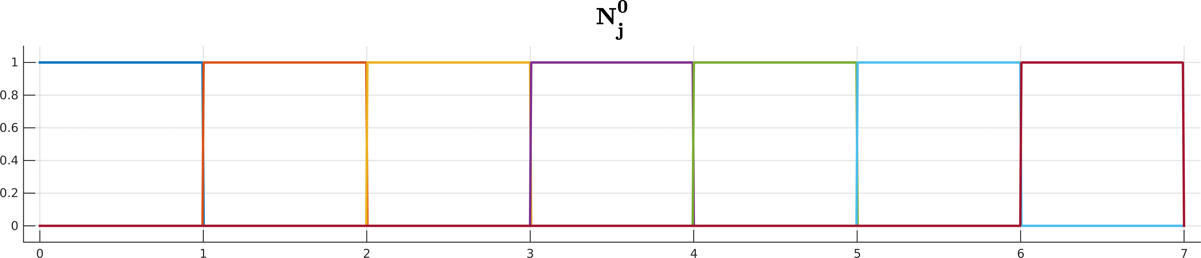
B-spline basis functions $N^k_j$ up to degree 5 for the knot sequence $(0,1,2,3,4,5,6,7)$.
De Boor’s algorithm
… also called the De Boor-Cox algorithm can be seen as a generalization of the De Casteljau’s algorithm. (Bézier curve is in fact a B-spline with a special knot sequence.)
- input :
$\mathbf{d_{0}},\dots,\mathbf{d_{n}}$ : control points
$t_0 \leq t_1 \leq \dots \leq t_m$ : knot vector
$t \in [t_i, t_{i+1}) \subset [t_k, t_{m-k})$ where $k = m-n-1$ is the degree - output : point $\mathbf S(t) = \mathbf d_i^k$ on the curve
- algorithm : For $j=i-k, \dots, i,$ set $\mathbf d_j^0 = \mathbf d_j$. Then compute the points \begin{align} \mathbf d_{j}^{r} &= (1-w_{j,k-(r-1)}) \mathbf d_{j-1}^{r-1} + w_{j,k-(r-1)} \mathbf d_{j }^{r-1} \end{align} for \begin{align} \quad r = 1,\dots,k, \quad \quad j = i-k+r,\dots,i \end{align} with \begin{align} w_{j,k-(r-1)} &= \frac{ t - t_j }{ t_{j+k-(r-1)} - t_j }. \end{align}
Be careful with the indices! Here we have expressed a point at depth $r$ in terms of points at depth $r-1$ – that is why there is the $r-1$ everywhere in the formula.
This might be a bit annoying, but I think it’s also more practical for the recursive implementation. (The formula becomes much more elegant if we express level $r+1$ in terms of level $r$.)
A cubic B-spline with 16 segments and endpoint interpolation.
ToDo$^1$
- Implement the De Boor’s algorithm.
- Evaluate B-spline for the
simpledataset. Modify the knot vector and recompute. What changed? - Evaluate B-spline for the
spiraldataset. Modify the knot vector to0 0 0 0 1 1 1 1 2 2 2 2 3 3 3 3 4 4 4 4 5 5 5 5. What changed? - Evaluate B-spline for the
cameldataset. Move the front leg by changing the x-coordinate of the last control point to-1.5. Which segments of the curve have changed? Why?
NURBS
If you’ve tested with the circle.bspline dataset, you were probably dissapointed:
the resulting curve is far from being a circle.
Here’s the bad news: it’s mathematically impossible to represent circle as a B-spline. But, it is possible via a generalization called Non-Uniform Rational B-Splines or NURBS.
Why the long name? Non-uniform simply means the knot sequence is non-uniformly spaced. Rational means we work in homogeneous coordinates by assigning a weight to each point.
In plane, the point $(x,y)$ becomes $(x,y,1) \approx (wx,wy,w)$.
If you examine circle9.nurbs file, you’ll it’s quite similar to circle.bspline.
The only thing that’s changed is the addition of a third coordinate – this is the weight w.
And here’s the good news: even with the homogeneous coordinates, we can apply exactly the same De Boor’s algorithm without any modifications!
Here’s a secret recipe for transforming your B-spline code to work with NURBS:
- The columns of
ControlPtsread from a.nurbscorrespond tox,yandw. Therefore, you first need to multiply bothxandy(columns 0 and 1) byw(column 2). - Feed the homogeneous control points
[w*x,w*y,w]to the De Boor’s algorithm you’ve implemented previously. - Convert the computed points (stored in the matrix
Segment) back to Cartesian coordinates. Divide by the third column to pass from[w*x,w*y,w]to[x,y,1]. - As before, plot the first two coordinates.
Hint: in Python, the operators * and / are applied element-wise, so you can do stuff like
matrix[:,0] *= matrix[:,2]
matrix[:,0] /= matrix[:,2]
ToDo$^2$
- Modify your code to work in homogeneous coordinates (if
dim=3). - Evaluate
circle9.nurbsandcircle7.nurbs. Compare the results withcircle.bspline.
Resources
- B-spline and De Boor’s algorithm
- 1.4.2 B-spline curve and 1.4.3 Algorithms for B-spline curves, online chapters from the book Shape Interrogation for Computer Aided Design and Manufacturing by N. Patrikalakis, T. Maekawa & W. Cho
- NURBS on wikipedia (includes the circle example)
- homepage of Prof. de Boor