TP6 : Bézier Surfaces

Code

• TP6 on github
• general instructions

Tensor-product Bézier surfaces

Tensor product Bézier surfaces are a direct generalization of Bézier curves. Instead of a control polygon $\mathbf b_i$, we consider a control net $\mathbf b_{ij}$. A Bézier surface is the described as

\[S(u,v) = \sum_{i=0}^{m} \sum_{j=0}^{n} \mathbf b_{ij} B_{i}^{m}(u) B_{j}^{n}(v)\]

where $m,n$ are degrees in $u,v$, respectively; $B_{l}^{k}$ are Bernstein polynomials.

Evaluation

To evaluate a point $S(u,v)$ on a surface, let’s fix $j$ and vary $i$.

\begin{equation} \displaystyle B(u,v) = \sum_{j=0}^{n} B_{j}^{n}(v) \underset{= \mathbf b_{j}(u) } { \underbrace{ \left[ \sum_{i=0}^{m} \mathbf b_{ij} B_{i}^{m}(u) \right] } } \end{equation}

The $\mathbf b_{j}(u)$ defines a Bézier curve in $u$ and can be evaluated using the De Casteljau.

\begin{equation} \displaystyle B(u,v) = \sum_{j=0}^{n} \mathbf b_{j}(u)B_{j}^{n}(v) \label{final} \end{equation}

This equation defines a Bézier curve in $v$ with control points $\mathbf b_{j}(u)$ depending on $u$. At the end of the day, we have

• $n+1$ evaluations of the De Casteljau for the degree $m$;
• $1$ evaluation of the De Casteljau for the degree $n$.

Alternatively, we can fix $i$ and vary $j$.

Bézier patch evaluation scheme. (image by Pierre-Luc Manteaux)

Coordinate matrices

In the code, the control points $\mathbf b_{ij}$ are actually stored in three coordinate matrices $\texttt{Mx}, \texttt{My}, \texttt{Mz} \; $ so that

\[\mathbf b_{ij}^x = \texttt{Mx(i,j)}, \qquad \mathbf b_{ij}^y = \texttt{My(i,j)}, \qquad \mathbf b_{ij}^z = \texttt{Mz(i,j)}.\]

This means the code is more comprehensible as the structure of the matrices directly represents the grid topology of the patch. On the other hand, it also means the computation needs to be done for each coordinate individually.

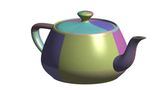
Bézier surface vs. piecewise Bézier surface

In practice, a Bézier surface often consists of multiple surface patches, each having its own control polygon. Therefore, it is sometimes called a piecewise Bézier surface.

Some surfaces in the data/ folder consist of more than one patch, ranging from 2 (heart) to 32 (teapot). They are saved in the BPT format; some datafiles are taken from the website of Ryan Holmes where you’ll also find more details about this format in case you’re interested.

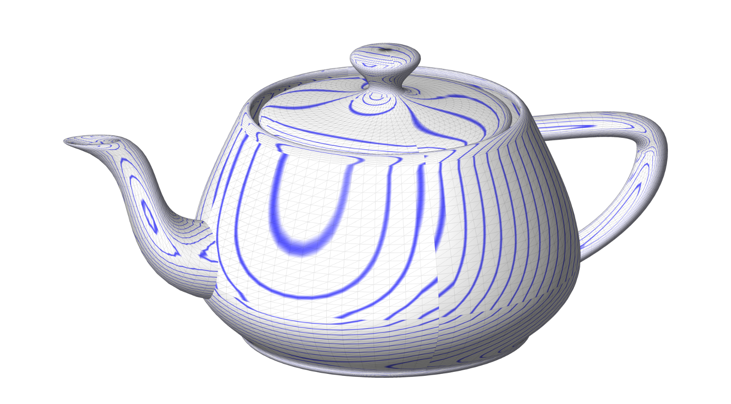
The discontinuity in isophotes shows the piecewise Bézier Utah teapot is not $\mathcal C^1$.

ToDo

1. Implement the evaluation of Bézier surfaces for $(u,v) \in [0,1]^2$. Use simple and wave for first tests (these contain only one patch).
2. When you’re sure the implementation works for the simple cases, test your algorithm on datasets with multiple patches: heart (2), sphere (8), teapot (32), teacup (26), teaspoon (16). Don’t set the density parameter too high, always start with smaller values (5 or 10) as the number of computed points is density².

Resources

• the website of Ryan Holmes with Bézier surfaces as BPT files
• Bézier surfaces on wikipedia
• construction and properties of Bézier surfaces by prof. Ching-Kuang Shene