TP4 : Subdivision curves

3 March 2017 in

Code

Subdivision Curves

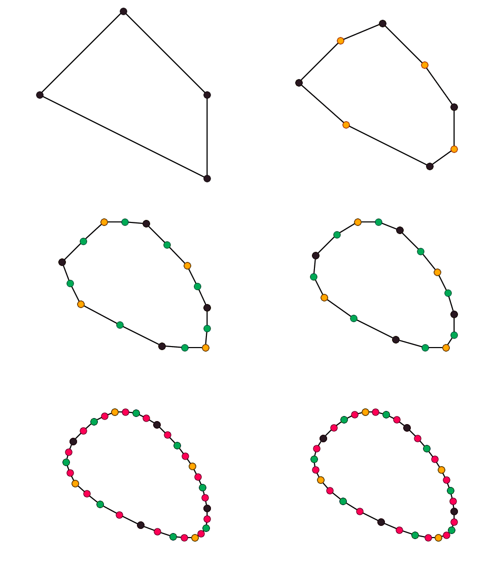
A subdivision curve is defined as the limit of recursive refinement of the input polyline $\mathbf x_i = \mathbf x_i^0$. Your today’s task is to implement three curve subdivision schemes from the lecture. For the sake of simplicity, we’ll be working with closed curves only.

Generally, one iteration of curve subdivision has the following form:

Topological step: curve is upsampled by inserting a new vertex between each two adjacent vertices. This doubles the number of vertices: if there were $n$ vertices, now there is $2n$ of them.
Geometric step: new positions are computed for all vertices.

subdivision-animation

There are two kinds of schemes: approximating schemes change the positions of old vertices, while the interpolating schemes don’t.

Chaikin’s scheme

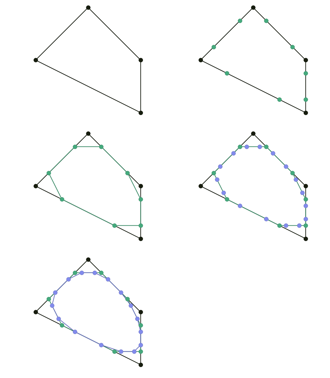
Introduced in 1974 by George Chaikin, this algorithm revolutionized the world of numerical geometry. Limit curve is a uniform quadratic B-spline.

\[\left\lbrace \begin{align} \mathbf x_{2i }^{k+1} & = \tfrac34 \mathbf x_i^k + \tfrac14 \mathbf x_{i+1}^k \\ \mathbf x_{2i+1}^{k+1} & = \tfrac14 \mathbf x_i^k + \tfrac34 \mathbf x_{i+1}^k \end{align} \right.\]

chaikin-scheme

Corner-cutting

Generalization of Chaikin’s algorithm with two parameters $ 0 < a < b < 1 $.

\[\left\lbrace \begin{align} \mathbf x_{2i }^{k+1} & = (1-a) \mathbf x_i^k + a \mathbf x_{i+1}^k \\ \mathbf x_{2i+1}^{k+1} & = (1-b) \mathbf x_i^k + b \mathbf x_{i+1}^k \end{align} \right.\]

Setting $a=0.25, b=0.75$ gives Chaikin. The following example uses $a = 0.1, b = 0.6$:

4-point

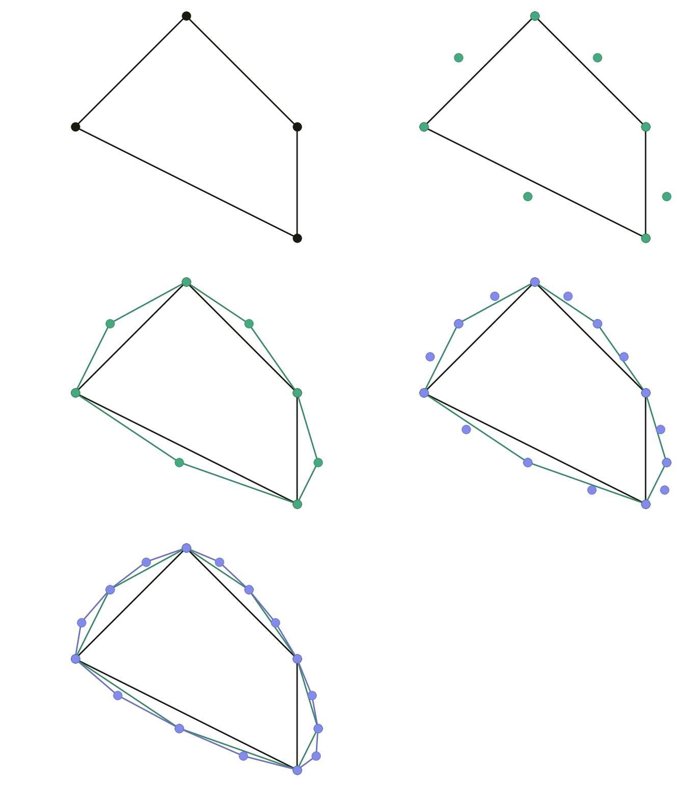
Four-point

Unlike corner cutting, the four-point scheme is interpolatory.

\[\left\lbrace \begin{align} \mathbf x_{2i }^{k+1} & = \mathbf x_i^k \\ \mathbf x_{2i+1}^{k+1} & = \tfrac1{16} \left( - \mathbf x_{i-1}^k + 9 \mathbf x_{i}^k + 9 \mathbf x_{i+1}^k - \mathbf x_{i+2}^k \right) \end{align} \right.\]