TP5 : Lane-Riesenfeld algorithm

Code

• TP5 on github
• general instructions

Uniform B-splines

In TP3, you have implemented the De Boor’s algorithm for evaluation of general B-splines. Now, let’s have a look at a particular subclass of B-spline curves, characterized by the uniform knot vector $t_i = i \; \; \forall i \in \mathbb Z$; have a look at the basis induced by such vector.

Your today’s task will be to implement these uniform B-splines as subdivision curves.

Lane-Riesenfeld algorithm

For a given degree, the following constitutes one subdivision step of the Lane-Riesenfeld algorithm. From initial polygon $\mathbf P_0, \mathbf P_1, \dots, \mathbf P_{n-1}$ with $n$ vertices, we compute subdivided polygon $\mathbf S_0, \mathbf S_1, \dots, \mathbf S_{2n-1}$ with $2n$ vertices.

Double the points (refining) :

\[\begin{align} \mathbf V_{2i}^0 &= \mathbf P_i \\ \mathbf V_{2i+1}^0 &= \mathbf P_i \quad \quad \text{for} \quad i=0,\dots,n-1 \end{align}\]

Average multiple times (smoothing) :

($i$-indices are taken modulo $2n$)

\[\begin{align} \mathbf V_i^d = \frac12 \left( \mathbf V_i^{d-1} + \mathbf V_{i+1}^{d-1} \right) \quad \quad & \text{for} \quad i=0,\dots,2n-1 \\ & \text{and} \quad d=1,\dots,\text{degree} \end{align}\]

Replace :

\[\mathbf S_i = \mathbf V_i^{\text{degree}} \quad \text{for} \quad i=0,\dots,2n-1\]

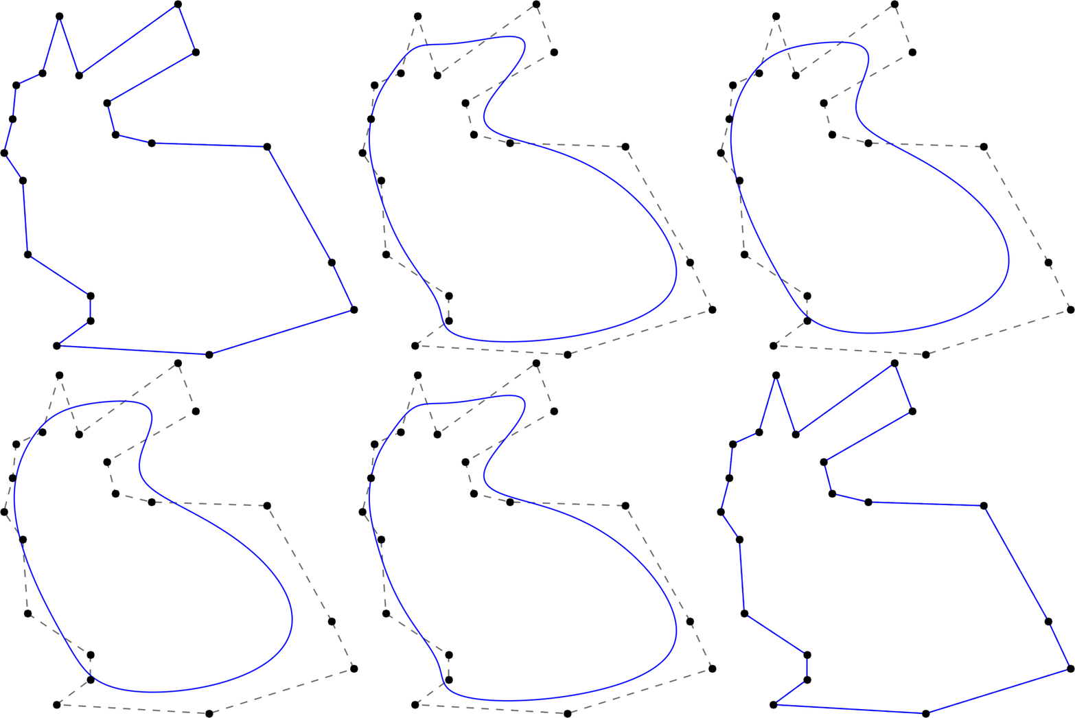
With increasing degree, the Stanford bunny becomes smoother and smoother. Here, the degree runs from 2 to 20 and back.

Variations on the Lane-Riesenfeld algorithm

Since the introduction of the algorithm by Lane and Riesenfeld in 1980, multiple variations of the original scheme were introduced. We will implement two of them, replacing the midpoint averaging with four-point and six-point averaging. You already know the four-point averaging from the previous TP.

For brevity, I’m only including the modified parts of the original algorithm.

Don’t forget the indices are taken modulo $2n$ in the smoothing step!

Four-point

In the refining step, vertices are no longer doubled: the new ones are already computed via four-point averaging. Then, we perform additional degree averagings on all vertices.

Refine :

\[\begin{align} \mathbf V_{2i}^0 &= \mathbf P_i \\ \mathbf V_{2i+1}^0 &= \tfrac{1}{16} \left( -\mathbf P_{i-1} + 9\mathbf P_i + 9\mathbf P_{i+1} - \mathbf P_{i+2} \right) \end{align}\]

Smooth :

\[\begin{align} \mathbf V_i^d = \tfrac{1}{16} \left( -\mathbf V^{d-1}_{i-1} + 9\mathbf V^{d-1}_i + 9\mathbf V^{d-1}_{i+1} - \mathbf V^{d-1}_{i+2} \right) \end{align}\]

Six-point

Very similar to the four-point scheme.

Refine :

\[\begin{align} \mathbf V_{2i}^0 &= \mathbf P_i \\ \mathbf V_{2i+1}^0 &= \tfrac{1}{256} \left( 3\mathbf P_{i-2} -25\mathbf P_{i-1} + 150\mathbf P_i + 150\mathbf P_{i+1} -25\mathbf P_{i+2} +3\mathbf P_{i+3} \right) \end{align}\]

Smooth :

\[\begin{align} \mathbf V_i^d = \tfrac{1}{256} \left( 3\mathbf V^{d-1}_{i-2} -25\mathbf V^{d-1}_{i-1} + 150\mathbf V^{d-1}_i + 150\mathbf V^{d-1}_{i+1} -25\mathbf V^{d-1}_{i+2} +3\mathbf V^{d-1}_{i+3} \right) \end{align}\]

ToDo

1. Implement the three subdivision schemes (for closed polygons). Test with the provided datasets.
2. Try varying the degree parameter. How do the curves change?
3. What differences between the three schemes do you observe? In your opinion, which scheme gives better results? Why?
4. Simplify the original Lane-Riesenfeld scheme for degree=2. What do you observe?

Resources

• Subdivision curves on Numerical Tours by Gabriel Peyré
• Subdivision spline curves
• Generalized Lane–Riesenfeld algorithms, paper by Cashman et al. (CAGD 2013)
• A Six-Point Variant on the Lane-Riesenfeld Algorithm, paper by Ashraf et al. (JAM 2014)